Reconstructing graphs from a digitally scanned plot

Nowadays, journals and articles are released online which can easily be downloaded by the readers. These include plots and figures in a digital form. In the past, however, the construction of plots in journals and articles are oftentimes hand-drawn. If suppose you need to incorporate the plot from a very old reference, digital scanning and reconstruction of plots from a digital copy can be applied to be able to extract the information (eg, plot) and be able to use it in a digital form.

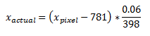
Figure 1 is an example of a digitally scanned hand-drawn graph obtained from a thesis manuscript published on the year 1980 [1]. In reconstructing plots from a digital copy, it is important that the original copy contains the correct coordinate label. Using the software GIMP or Paint (in my case, I used paint), we can extract the pixel values of each point in the plot and derive an equation that would relate the pixel value to its corresponding actual value in the plot. The good thing about my image is that, it already contains grid that guide the readers about its coordinate.

Figure 1. Digitally scanned copy of a hand-drawn plot from a thesis manuscript

My first thoughts regarding the problem involves obtaining enough number of data points (pixel values) from the plot and then find an equation that would relate the pixel values to the actual values. At first, I was thinking of using the pixels at the origin as my point of translation. Since the origin of the plot is located at a pixel value x equal to 781 and a pixel value y equal to 2469, I could just use these as my reference so that the equations that would relate the actual values to the pixel values are the following:

The fraction 0.06/398 are obtained by determining the number of pixels between each grid in the plot. From figure 1, the number of pixels in each 0.06 intervals in the x-axis are averaged. The same method was done for the y-axis.

The following figure displays the result of the image reconstruction with the original image overlaid with the reconstructed plot. In overlaying the images, it is important that the origin and the maximum value of the plot follows that of the reconstructed so that there is no induced bias in comparing the plots. This can be done by cropping the plot from the original image and then use it as a background for the plot in excel. I would like to thank Alix for teaching me how to overlay the images. :)

Figure 2. Reconstructed plot using translation of origin

The problem I encountered in the first method was that the image I obtained is not perpendicularly scanned. With the use of GIMP, the image was gradually rotated. I tried to get the correct angle that should be used to rotate the image to obtain a perfectly perpendicular image, and that is just by taking the x and y pixel values of the y-axis and then use the known trigonometric identities (arctan).

Later did I realize that I could actually convert each pixel value to its corresponding actual value and then I could obtain an equation that would relate them with the use of a linear regression since I have a set of pixel and actual values. I was not really paying enough attention to what was discussed by Dr Soriano during class, so it was only just during the time that I was writing this blog that I realized that linear regression of the pixel and actual values is more straightforward and is easier. And then it occurred to me that she wrote something at the board about obtaining an equation of a line that relates the pixel and actual values for both x and y axes. That's it! It all made sense now :D

With the use of the pixel values of all labeled coordinates extracted from each axis of the plot, I obtained a linear regression of the actual x values and y values of the plot in relation to its x pixels and y pixels, respectively. This together with the equation of the linear regression is shown in the following figure. To be able to obtain a larger number of data points for the y-axis, I counted the number of grid displayed on Paint between values 0.5 and 1.0 and then I divided it to two to obtain a pixel value for 0.75. This was also done to obtain a pixel value of 0.25. 

Figure 3. Pixel conversions in both x and y axes obtained using linear regression

The x and y pixel values of points in the plot are tabulated. It is not necessary that we obtain all pixel values that corresponds to the plot. In my case, I only obtained 88 x and y pixel values. This part of the experiment is the most exhausting since it requires the use of two programs simultaneously (excel for recording and paint for pixel value extraction). I suggest that you you either minimize the size of the windows for each application or use only the 2 programs needed so you could easily switch from one application to another.

Using the equations obtained using the linear regression, the pixel values extracted are then converted to their actual values. Finally, the points are plotted and the digitally scanned copy is overlaid at the background. The result is shown in figure 4.

Figure 4. Reconstructed plot using linear regression of pixel-value conversions

Based from the results, we could see that there's really no significant difference between the two methods. When the fraction (pixel conversion) in the equations proposed in the first method is distributed such that the equation follows the slope formula, it basically reduces to an equation almost the same from the result of the linear regression. Having accomplished both methods, I could say that the second method is more straightforward than the first, since you need not obtain the pixel value of the origin as long as you have the correct x and y axis pixel to actual value conversion.

I remember doing this activity in my 3rd year as part of my skill building training for research when I was freshly admitted from the Instrumentation Physics Laboratory. Back then, I only used the second method, and it was a little exhausting. Overall, I would give myself a grade of 11/10.


References:
[1] Domingo, Zenaida (1980) Computer simulation of the focusing properties of selected solar concentrations, M.S. Thesis. UP Diliman
[2] M. Soriano. Applied Physics 186 Manual A2 - Digital Scanning