Learning Scilab

One of my research problems involves processing of images obtained from my experiments on granular flow, and my adviser suggested that I use Scilab or Matlab since they are more inclined to be used when performing many different image processing techniques.

Today's activity is about the basics of Scilab. By the end of the meeting, we were required to display the plots of the following:
 a. centered square aperture
b. sinusoid along the x-direction (corrugated roof)
c. grating along the x-direction
d. annulus
e. circular aperture with graded transparency (Gaussian transparency).

The first part which is the centered square aperture is more straightforward than the given example which is the centered circle. Figure 1 shows my plot together with the code I used. In my code, there is a luxury to change the width of the square as long as the preferred width is less than 2.

figure 1. Squares of different width

I had to search what corrugated means when I came to know that I have to create a sinusoid along the x-axis with a corrugated roof. Since it is a sinusoid, it is natural that a sine or cosine function is involved. Shown in the following figure is an image of the generated sinusoid with different frequencies. The image shown is the top view of the figure shown just below it.

Figure2. Sinusoids of different frequency with corrugrated roof

Figure 3. 3-D image of the generated sinusoid

I had a hard time generating the image of a grating just because I used the wrong way of plotting. I already thought about using the same technique with the one I used in generating the sinusoid. I used the code 

f = scf();

grayplot(x,y,A);

f.color_map = graycolormap(32);

but I ended up having a grading but with shades of gray at the edge of every color as shown below:

Instead of using this code, I just used imshow and voila, I was able to eliminate the gray colors. :) The generated images are shown in Figure 4. I used different frequencies to vary the number of gratings.

Figure 4. Gratings of different frequencies

In generating the annulus, I just introduced a small variation in the original code of the circular aperture. Shown in Figure 4 is the result of varying the inner and outer radius of the annulus. Instead of converting all values below a certain radius (outer), we restrict the change of values up to a certain smaller radius only (inner radius). 

Figure 5. Annuli of different inner and outer radii

The last figure to be generated is the circular aperture with graded Gaussian transparency. This part was a little more challenging than the previous images since it requires a Gaussian transparency gradient. 

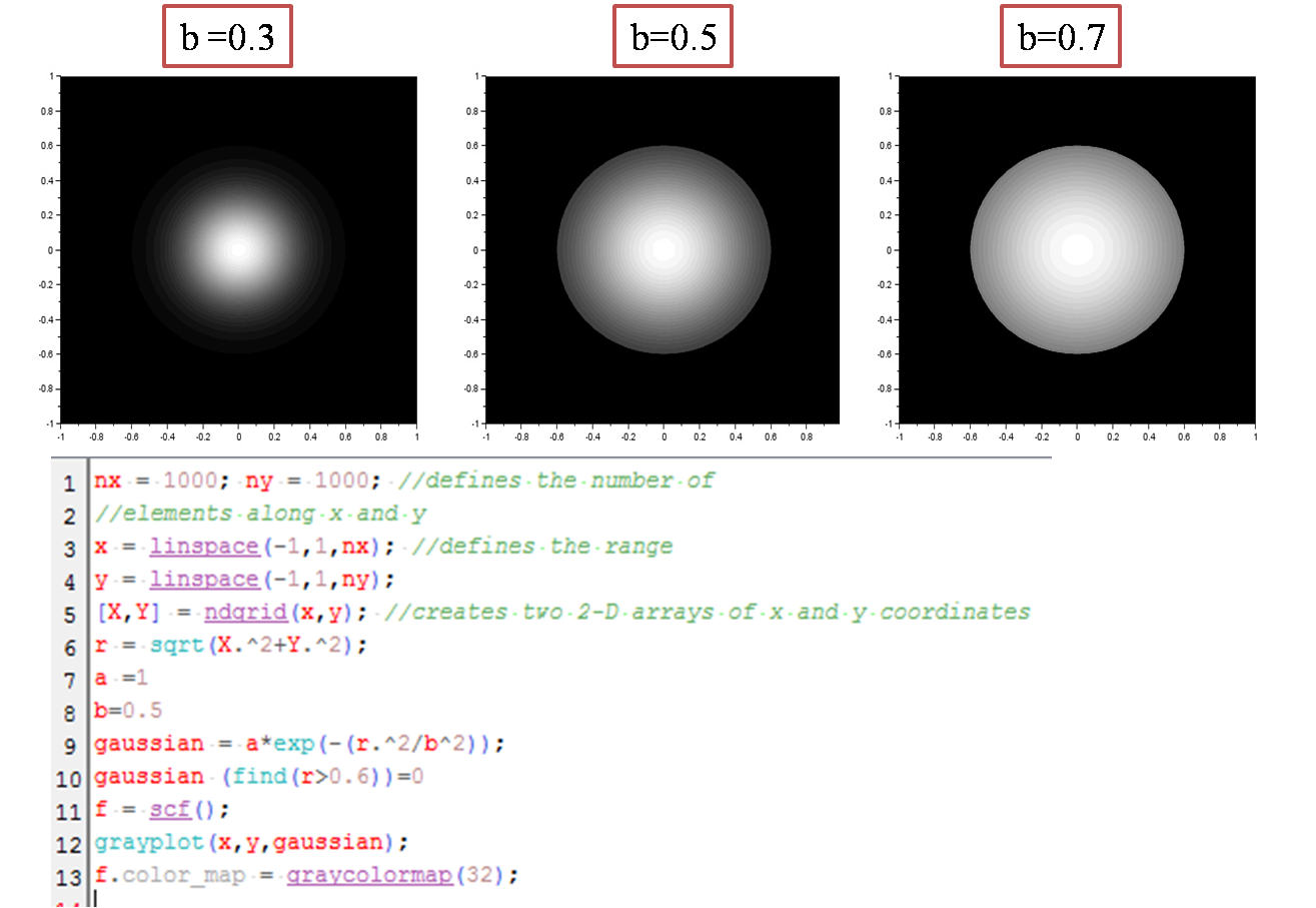
Figure 6. Circular apertures of different graded transparency with radius =0.6

The last part leaves the students to explore more about the possible images that can be generated when combining the different techniques used in generating the different shapes. I was able to generate the following images:

I tried multiplying the matrices element by element and this is what I got. Quite cute! :D

In this last part, I explored the syntax mesh and randomly applied it to my code in generating a circular aperture with a graded gaussian transparency. Voila! :D

I enjoyed this activity and I'm looking forward to learning more programming techniques. :) Overall, I give myself a grade of 12/10 for exploring several parameters that could vary the resulting image.