Image enhancement using histogram manipulation

The next task for our 186 lab class is image enhancement using histogram manipulation. Based from experience, we sometimes fail to set the correct settings in our camera before capturing a scene. Most of the time, (well in my case and based from my own observation and experience), it is a common mistake to take a shot that is dark. There is a certain threshold to which our eyes is sensitive to. In this activity, we can enhance dark images to be able to see more detail about the picture.

I chose the following image of Aeriel during her mock wedding with Nestor last February. As you can see, the image is dark and the objects in front of Aeriel are not clear. Now, suppose we want to enhance the image to make it look brighter and more detailed, we could just manipulate the grayscale PDF of the original image by backprojecting the grayscale values of a desired cummulative distribution of grayscale values.

Image to be enhanced

The first step is to get the cumulative histogram (CDF) of the grayscale values of the image and use it to backproject values from the desired one. The CDF of a normal probability distribution function is that of a constant. So in enhancing our image, our goal is to normalize as much as possible the histogram of our image.  The following image shows the original and the enhanced CDF of our image.

As observed, the highest pixel value present in the original image is only about 100 pixels, which is why the image is generally dark.  Recall that in a grayscale image, the brightest pixels are at 255 px. I started by converting a given RGB image into grayscale and plotted its histogram. I then proceeded to computing its CDF and as already mentioned, the result is shown in the left side of the above picture. 

Using the  original and the desired CDFs, the pixel values of the grayscale image is replaced. I remember our 185 class and thought about the input-output curve of a system. In this case, the I-O curve is the desired CDF.

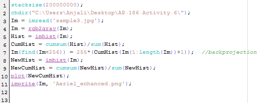
I was not really familiar with the matrix operations here in Scilab and I first opted in using for loop. But then my code was not working and for some reason I couldn't find the bug. Aside from the fact it is slow and faulty, it was not elegant. So then Joshua thought me with the one-line code. I didn't know that Scilab allows operations in each element of a matrix to be done simultaneously. Although the idea is the same, mine was broken down to for loop, where the operation is performed to each element one at a time. I was amazed when I found out that Scilab could handle a matrix operation as one. Indeed, it could be the best tool for image processing.

Finally, I produced the following enhanced image:

Wondering what happened to the histogram of the enhanced image? Here:

Histogram of the enhanced image

Observing it closely and comparing it to the original histogram, I realized that the the points were just basically spread out through the 1-255 range. It was made to follow the normal distribution. Its cumulative distribution is quite more interesting since it wasn't able to follow an exactly straight line. Shown below is the CDF of the enhanced image and the desired (straight line).

CDF of the enhanced image

This method here can also be done without using Scilab. Other free and more user-friendly software are available online. One example is the GIMP. We can use GIMP to manipulate the histogram of a given image the same way we did using Scilab. Now loading the same image in GIMP and following Image > Mode> Grayscale and then Color > Curves, we can adjust the color curves of the image by choosing the preferred input-output curve. In our method using Scilab, we chose a constant line as our I-O curve. A snapshot of the manipulation using GIMP is shown below:

Histogram Manipulation using Color Curve in GIMP (Grayscale)

One also has the option to do this without converting the image to grayscale. The different channels red, green and blue can be manipulated individually as can be seen from the snapshot below:

Histogram Manipulation using Color curve in GIMP (RGB)

This technique can also be done by using other softwares like Photoshop. Here one can simultaneously view the resulting histogram of the image as you vary the I-O response curve. The picture below shows a snapshot of the Curve and the Histogram of the same image loaded to Photoshop.

Histogram Manipulation using Photoshop

Indeed, there are a lot of techniques available in enhancing an image. It is interesting to understand how these software work. Behind their user-friendliness is a deep information that only lucky students like us can be able to understand. For this activity, I give myself a grade of 11/10 for doing all the required work and for further exploring other software. I am looking forward to the next activities. :)